


Microsoft Excel has traditionally been the go-to tool for data analysis due to its versatility and user-friendly interface. It enables users to conduct complex calculations, statistical analysis, and data visualization without requiring advanced programming skills. However, over time, it has slowly started losing its throne to Pandas, at least in some companies.
Although Pandas requires users to invest time in learning Python programming, this investment is minor compared to the significant advantages it offers over Excel. These benefits include efficient handling of large datasets, faster processing speeds, greater flexibility, simplified automation of tasks, and smooth integration with machine learning algorithms. As a result, many professionals have transitioned to Pandas to make use of its powerful capabilities.
Initially, it seemed inevitable that Excel would remain behind. However, the developers of Excel introduced a game-changing idea: integrating the power and flexibility of Python and Pandas directly into Excel.
In a previous article, we covered the fundamentals of using Python within Excel. Now, we will take a closer look at whether integrating Python into Excel can fully replicate the advantages of Pandas.
What Are the Differences between Python in Excel and Pandas
The simplest method to evaluate if Python in Excel matches the feel and functionality of Pandas in Python is to compare specific operations in both environments. However, this comparison might be somewhat misleading since Python integration in Excel allows users to import Python libraries just as they would in a standard Python file. Notably, one of these libraries is Pandas itself. Therefore, the comparison of Python in Excel with standard Pandas in Python environments becomes more complex. Essentially, it turns into a comparison between using Pandas directly from Excel and using it traditionally, such as running code in a Jupyter Notebook.
Since the code itself remains consistent whether executed in Python cells within Excel or code cells in a Jupyter Notebook, there is little to compare in terms of the code itself. Instead, the key comparison lies in the results generated by these two different environments. Specifically, Python code in Excel runs on Microsoft Azure in the cloud. Therefore, we will evaluate the outputs from both environments. The purpose of this is to determine if using Pandas from Excel is as efficient as running Pandas code in a Jupyter Notebook or if it falls significantly short.
How to Effectively Examine and Represent Data
When analyzing and processing data with Pandas, the initial step is usually to load the data and create a DataFrame. This process is quite simple, typically achieved using a single function in Pandas. The specific function depends on the file type of data. However, no matter the type of data, all we usually need to do is write a single line of code. For instance, to read data from an Excel file we would use the read_excel function, while for a CSV file, we would use the read_csv function, and so on.
In Excel, our data is already “loaded in”. To be more precise, in Excel, we work with spreadsheets that contain columns, rows, and cells where our data is already stored. Therefore, there is no need for any type of explicit data-loading process. However, there is an additional step to it. If you want to apply Pandas DataFrame methods for data processing, you first need to create a DataFrame from the data in your worksheet.
In this article, to demonstrate the usage of Pandas in Excel, we will work with the survey_sample.csv file. You can download this file by going to this link:
https://edlitera-datasets.s3.amazonaws.com/survey_sample.csv
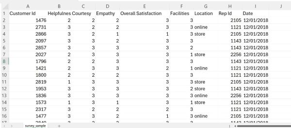
Once you do so, just open the file with Excel. This is how the data in the file looks like:
As can be seen, we have the following columns:
- Customer Id
- Helpfulness
- Courtesy
- Empathy
- Overall Satisfaction
- Facilities
- Location
- Rep Id
- Date
The file contains ratings of sales representatives based on their skills, as well as ratings of overall customer satisfaction with the service and the facilities. Before we begin analyzing the data, we will create a Python cell to import the Pandas library. Libraries in Python are usually imported at the top of the code. Since code gets executed from top to bottom, importing libraries that we plan on using at the top helps prevent errors later in the execution.
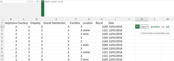
To import Pandas, click on a cell near our data, in the top row, convert it into a Python cell, and then just type in the necessary code:
When using libraries in Python it is common to import libraries under an alias, because we often need to type in the library name to invoke certain functions from it. Pandas is usually imported under the alias pd because that significantly shortens how much code we need to write. Yet, it remains descriptive enough for others to understand which library is being used.
Because Excel automatically displays the output of the code executed you will see None when importing a library. The operation of importing a library enables us to use that library, but in essence, there is nothing returned. So if you successfully imported Pandas, the cell should return None:
As a warning, most data processing libraries and visualization libraries are already preloaded. In other words, there is no need at all to import Pandasat to use it. However, in case you want more niche libraries, you will need to import them as demonstrated above.
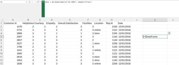
With Pandas ready, we can go ahead and create a DataFrame from our data. To achieve this, we can simply use the DataFrame constructor from Pandas, specifying the data from the worksheet as the source for creating the DataFrame:
Now that the DataFrame has been created and stored inside the data variable, we can start performing operations on it. The simplest operation we can perform is just taking a look at the DataFrame itself. To be more precise, let us use the head() method to display the first five rows of the DataFrame:
This is the time to mention that there are two modes for running this code in Excel. By default, when you run the code in Excel, it returns the object resulting from the code execution. For instance, using the head() method will return a DataFrame containing only the first five rows of the main DataFrame. However, Excel does not display this new DataFrame directly. To display the DataFrame in the Excel cell rather than just showing the object type, you need to use the small toolbar next to the formula bar in Excel. Select that you want Excel to return as output NOT the Python object, but instead the Excel value:
When you select that, the code is going to run again, but this time you will get a display of the object (in this case DataFrame):
As can be seen, we get a good display of the first five rows of our DataFrame. Comparing the first five rows here with the first five rows in the columns we have in the worksheet, you will notice that the data is identical. In other words, we successfully created a DataFrame from the data stored in the worksheet.
Article continues below
Want to learn more? Check out some of our courses:
How to Compute Statistics Using Pandas in Excel
To be fair, displaying our DataFrame and selecting data within is not the primary reason for using Pandas in Excel. After all, we can already see what our data looks like because it is there in our worksheet. Furthermore, some simple operations such as sorting and filtering are also easily performed in Excel. Therefore, there is no real benefit to focusing on these aspects. Instead, let us demonstrate the true power of Pandas in Excel by exploring two important methods that enable detailed data analysis with just a single line of code:
- info() method
- describe() method
How to Perform a Basic Analysis of Our Data
Using the info() method we can perform a basic analysis of our data. To be more precise, we can find out the following:
- the number of rows and columns in the dataset, i.e. the total number of data points
- the type of data we have in each column
- the amount of memory utilized by our dataset stored in a DataFrame
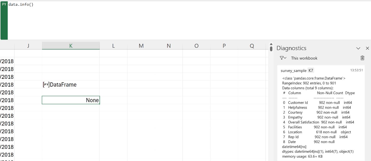
To use the info() method, we just need to apply it to our data stored in the DataFrame. The result we will get looks like this (keep in mind to set up the calculation so that it returns Excel values, and not a Python object, the same way we did when we used the head() method):
As can be seen, certain outputs that have quite a particular format in Pandas will be displayed in the Diagnostics window. This is the same window where we would usually be warned about errors in our Pandas code. From the display in the Diagnostics window we can infer the following:
- there are 902 rows and 9 columns in our dataset
- seven columns contain numerical data
- one column contains strings i.e. text
- there is one column that contains timestamps
- the “Location” column is missing some data
- this DataFrame takes up approximately 64 KB of memory
That is an abundance of useful information we receive from just running a single line of code. Finding out all of this information in Excel would take us far longer.
How to Calculate Descriptive Statistics
A particularly useful Pandas method is the describe() method. It helps obtain descriptive statistics about your dataset. By default, it computes statistics only for numeric variables, but it can be adjusted to include non-numeric variables as well.
For numeric data, the statistics included in the results are:
- Count: The number of entries in a column
- Mean: The average value across entries
- Std: Standard deviation, which measures the amount of variation
- Min: The smallest value
- 25%: The 25th percentile
- 50%: The median or 50th percentile
- 75%: The 75th percentile
- Max: The largest value
For non-numeric data, the statistics displayed are:
- Count: The number of entries in the column
- Unique: The number of distinct entries
- Top: The most frequent entry
- Freq: The frequency of the most frequent entry
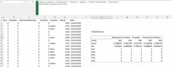
Let us first demonstrate the results we get when analyzing the numeric columns in our dataset. To be more precise, we will ignore the Customer Id and Rep Id columns when calculating statistics because those two represent identification numbers. Also, we will ignore the Date column because it contains timestamps. Finally, since the Location column contains text we will also ignore that column. To calculate descriptive statistics, we simply need to specify the columns of interest and after that use the describe() method on that part of our DataFrame:
Once again, calculating all of these values would take significantly longer if we didn’t use Pandas. This way, we can create a detailed statistical analysis of our data using a single method.
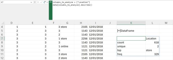
For the sake of demonstration, let us select just the Location columns as our column of interest to show how our result will look like when we analyze non-numeric data:
How to Merge Data from Different Sources
Frequently, we need to consolidate data from various sources before analysis. In Excel, merging two spreadsheets with overlapping columns typically involves using the VLOOKUP() function. While effective, this method isn't the most efficient, as it requires several steps to combine the datasets based on shared columns. Conversely, using Pandas in Excel can simplify this process significantly. We are going to merge the data we have in our spreadsheet with the data that can be found on this link:
https://edlitera-datasets.s3.amazonaws.com/survey_mappings.xlsx
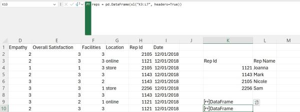
More precisely, we will merge our data with the data from the Reps sheet of the Excel file you can find on the link above. First, we will copy the data from that sheet to the one we are working with, and we will create a DataFrame from it. Let us call that DataFrame reps:
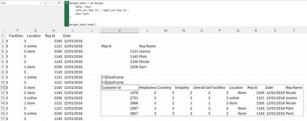
Now that our second DataFrame is ready, we can merge our two DataFrames using the merge() method from Pandas. To merge them using this method we just need to define which columns they have in common, and what type of merge we want to perform. In our case, we want to end up with a DataFrame that contains our original data together with a Rep Name column, a column that contains the names of the representatives connected to unique representative Ids. Therefore, we will perform a left merge based on the Rep Id columns in our two DataFrames. Let us also immediately display the first five rows of the resultant DataFrame:
As can be seen, we successfully merged the two DataFrames based on the information stored in the Rep Id column.
How to Summarize and Aggregate Data
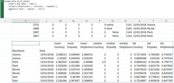
Pivoting data is a frequent task in Excel, typically involving numerous clicks and selections through various menus. However, when using the Pandas library in Python, this process can be streamlined significantly. With Pandas, the same result can be accomplished using a single line of code, albeit somewhat longer, by employing the pivot_table() method. Let us demonstrate how to calculate the mean, median, and standard deviation for each representative across two different years using this approach:
- define which columns we want to pivot around i.e. which columns we want to have in our index by defining them in the index argument of the method
- define the columns for which we want to calculate the mean, median, and standard deviation by defining them in the values argument of the method
- define that we want to calculate the mean, median, and standard deviation by defining them in the aggfunc argument in the method
As can be seen, creating a pivot table, even one where we pivot around multiple columns and in which we aggregate data using multiple functions is quite easy.
In this article, we demonstrated the simplicity and power of using Pandas directly within Excel. We showcased how simple it is to execute complex operations with this integration. While the efficiency gains may not be immediately apparent in our small sample of about 900 rows, the benefits of Pandas become much more significant as the dataset size increases. Pandas offers superior scalability compared to traditional Excel methods. Therefore, integrating Python and Pandas into Excel is more than just a novelty. Even in its current preview and beta-testing phase, it represents a substantial enhancement. This functionality is likely to become essential for Excel users in the future, revolutionizing how we approach data analysis within spreadsheets.

